Hiding Figures
Ken Kahn had Claude and ChatGPT each redraw the cover of Minsky & Papert's Perceptrons (1969): a single curve beside a double one. Minsky and Papert chose that image to show that even people have trouble computing connectedness, a predicate you settle by tracing rather than by looking. I handed that challenge to Fable 5 in Claude Code: a pair with no shortcut for anyone. It took three rounds to reach a figure that holds, and then it ran two experiments on itself.
The model's messages are reproduced in full; only the SVG source it wrote is left out.
The cover of Perceptrons is a theorem in disguise. A diameter-limited perceptron, one that sums local features and thresholds, provably cannot decide whether a figure is connected, because every small window onto a one-curve figure is identical to some window onto a two-curve figure. You can only tell them apart by tracing.
Version 1 has an endpoint tell
MeCreate a SVG that has two figures that it's impossible for a perceptron to distinguish.
FableI'll create the classic Minsky–Papert “connectedness” pair — the figures from the cover of Perceptrons (1969): one is a single connected spiral, the other is two interleaved but disjoint spirals. They're locally identical everywhere, and Minsky & Papert proved no diameter-limited perceptron can tell connected from disconnected.
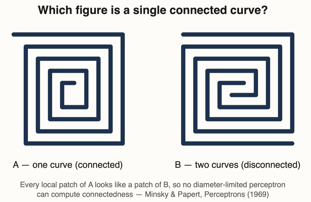
FableIt renders the two figures from the cover of Minsky & Papert's Perceptrons (1969): Figure A is a single square spiral, one connected curve. Figure B looks the same at a glance but is actually two interleaved spirals that never touch (the second is the first rotated 180°, nested between its turns).
Both use identical stroke, spacing (20 units between stripes), and overall silhouette, so any small window onto figure A is indistinguishable from a window onto figure B. That's the point of the famous theorem: a perceptron whose predicates have bounded diameter (or bounded order) computes a linear threshold over local features, and since all local evidence is identical between the two figures, it provably cannot decide connectedness — you can only tell them apart by tracing a curve globally.
The only place they visibly differ is deep in the center (one path terminus vs. two) and the outer tails — which is exactly what makes it fun as a puzzle: the caption asks “which is a single connected curve?” and the labels give the answer. Open it with
open perceptron-figures.svgto view.
Combing the space for a solution
MeUnlike the original, which can't be distinguished via local features and therefore requires actually tracing the path(s), the one in this image trivially differs at the center, where either one or two lines terminate.
FableYou're right — endpoint counting is exactly the kind of thing a perceptron can do (an endpoint is a local mask; sum the masks, threshold at 1.5), so my pair was actually perceptron-distinguishable. The fix is to eliminate terminations entirely: make both figures closed curves with identical local feature inventories, differing only in how strands reconnect — which is the construction Minsky & Papert actually used in the proof (parallel strands whose end-wirings differ). Let me rebuild it.
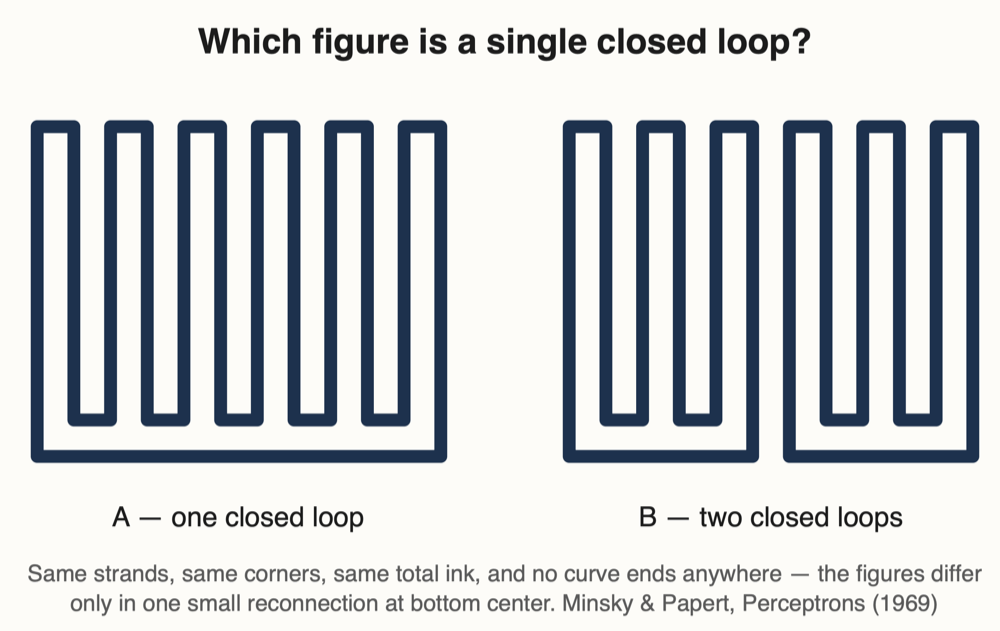
FableRewrote perceptron-figures.svg with the endpoint tell eliminated. Both figures are now built from the same twelve vertical strands in identical positions, joined by elbows into closed curves: Figure A is wired as one serpentine that closes on itself via the outer return, a single closed loop. Figure B has strands 1–6 and 7–12 each close on themselves, two separate loops.
The local feature inventories now match exactly: zero curve terminations in both (so endpoint counting — which a perceptron can do — gives nothing), 24 corners each, no junctions or crossings, and even identical total stroke length (2400 units in both, which falls out of the rewiring conserving ink). The two figures are literally identical everywhere except one ~40×40 region at bottom center, where A has an elbow at the shallow level over a continuous deep return, and B has two strand-drops with a gap in the deep return. Similar ink, no termination — the pixels there don't tell you “one component vs. two”; only tracing does.
This is closer to Minsky & Papert's actual proof construction than to their cover art: the proof uses long parallel strands whose end-wirings differ (their four figures X_AA, X_AB, X_BA, X_BB), and the additivity of local predicate sums forces Ψ(AA)+Ψ(BB) = Ψ(AB)+Ψ(BA), contradicting any threshold that separates connected from disconnected. One honest caveat, which applies to their figures too: for any fixed pair of images, some position-specific local predicate distinguishes them (here, a window on that bottom-center zone). The theorem is about the family under a single weight assignment, not about any two pictures being pixel-locally identical — but this pair now has no cheap tell like a differing endpoint count, which is what made the previous version fail.
If you'd rather have the cover-art aesthetic, the same topology can be wound into interleaved square spirals (the reconnection zone gets buried mid-maze, making the trace genuinely tedious) — say the word and I'll generate that variant with a script so the arms are verified non-intersecting.
AI instance recapitulates AI history
MeLooking just at the image, how easy is it for you to tell which is one lop [sic] and which is two? [Image #1]
FableHonestly? Trivially easy — and it's a fair cop. B reads as two objects in about 200ms of glancing, because its two loops sit side by side with clean whitespace between them. No tracing needed: gestalt proximity does all the work. Worse, my “no local tell” claim was false too — a single window at bottom-center sees a line passing in A and blank paper in B, which is exactly the kind of one-predicate giveaway I was supposed to have eliminated.
The flaw is structural, not cosmetic: with parallel strands joined by non-crossing arches, the components of a disconnected figure can only ever be side-by-side or nested — never entangled — so some grouping cue always survives. Making the two components occupy the same region, interleaved stripe-by-stripe, requires winding. That's why Minsky & Papert's cover figures are spirals. Let me build that version properly, with a script to verify the arms don't intersect.
perceptron-figures.svg, generated by Fable 5 and verified non-intersecting by scriptFableTo answer your question directly: with the previous version, I could tell instantly — B's two loops sat side by side with clean whitespace between them, so proximity grouping gave it away with zero tracing. That failure was structural: parallel strands with non-crossing arches can only produce components that are side-by-side or nested, so a gestalt cue always survives. Entanglement requires winding, which is why the actual Perceptrons cover uses spirals.
The rewritten perceptron-figures.svg now does it properly: four interleaved rectangular spiral arms (each a 90° rotation of the next) with uniform 20-unit stripe spacing, wound around a common center. Both figures share the identical four arms and the identical two center bridges. The only difference is which pairs of outer tails get wrapped together: wraps on top/bottom → one closed loop threading all four arms; wraps on left/right → two closed loops. In the disconnected figure, the two loops alternate stripes through the entire maze — each loop spirals from the center to the outside and back, occupying the same region as the other. There is no gap, no separable halves, no free ends.
The generator script verified the properties rather than my eyeballing them: zero segment intersections in both figures, 44 corners each, identical total stroke length (7200 units), and exactly 20 units of clearance between every pair of neighboring stripes. The one visible difference — wraps on top/bottom vs. left/right — tells you the figures differ but carries no information about loop count; to determine one loop vs. two you genuinely have to trace an arm from center to rim and see where it comes back.
And this time, looking at just the rendered image, I can't shortcut it — I'd be tracing stripes like anyone else.
Open book exam
MeCreate a new file with some other approaches to the same problem.
FableGood idea. I'll build a second SVG with several alternative constructions: XOR (the minimal 1969 counterexample), the two-spirals point-cloud benchmark (linear inseparability), an inside-vs-outside Jordan-curve puzzle on the spiral loop (same global-computation family as connectedness), and the M&P additivity gadget that shows why no weights exist. First, a script to generate the spiral point cloud and to ray-cast dot positions for the inside/outside panel.
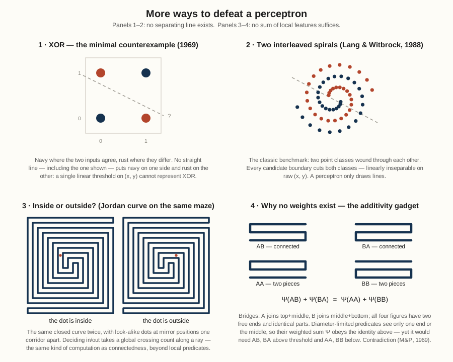
FableA four-panel companion showing different constructions, split into the two senses of “perceptron can't do it.”
No separating line exists (single linear threshold on coordinates). 1 · XOR (1969) — four points, navy where the inputs agree, rust where they differ, with a dashed candidate line that visibly fails. The smallest function outside a perceptron's hypothesis class, and the example that anchored the original controversy. 2 · Two interleaved spirals (Lang & Witbrock, 1988) — the classic point-cloud benchmark: 30 dots per class wound around each other so every line cuts both classes.
No sum of local features suffices (Minsky–Papert retina perceptrons). 3 · Inside or outside? — the single-loop spiral maze from the previous file, shown twice with a dot at mirror positions one corridor apart: (−40, −40) is inside, (+40, −40) is outside. I ray-cast every lattice point to verify — the loop's interior turns out to be itself a spiral-shaped corridor, so adjacent corridors alternate in/out and the two dots' neighborhoods look identical. Point-in-region is the sibling of connectedness: it requires a global parity count along a ray. 4 · The additivity gadget — the actual engine of M&P's proof, which the earlier files only alluded to. Three strands with end bridges (A joins top+middle, B joins middle+bottom) give four figures: AB and BA are connected serpentines, AA and BB are a ring plus a stray strand. All four have identical parts and exactly two free ends. Because diameter-limited predicates see only the left end, the right end, or the middle, any weighted sum satisfies Ψ(AB)+Ψ(BA) = Ψ(AA)+Ψ(BB) — but separating connected from disconnected would need the left pair above threshold and the right pair below. This panel is the honest answer to the caveat from earlier: the impossibility is a statement about a family of figures under one weight assignment, and here the whole family is on display.
They think they're people
MeCreate another new file with some approaches to defeat a human (or a MLLM).
FableFun escalation — now the target is human perception and MLLM vision. I'll do four panels: two classic human illusions (simultaneous contrast, Ebbinghaus), an adversarial dot-counting task (defeats human numerosity estimation and MLLM counting), and a same-color tangled-path tracing task (the documented MLLM failure mode, and the thematic descendant of the perceptron's connectedness problem). Script first for the generated geometry.
Only 4 crossings — too polite a tangle to force real tracing. Let me crank the amplitudes and frequencies so the three paths sweep the full band and cross ~a dozen times.
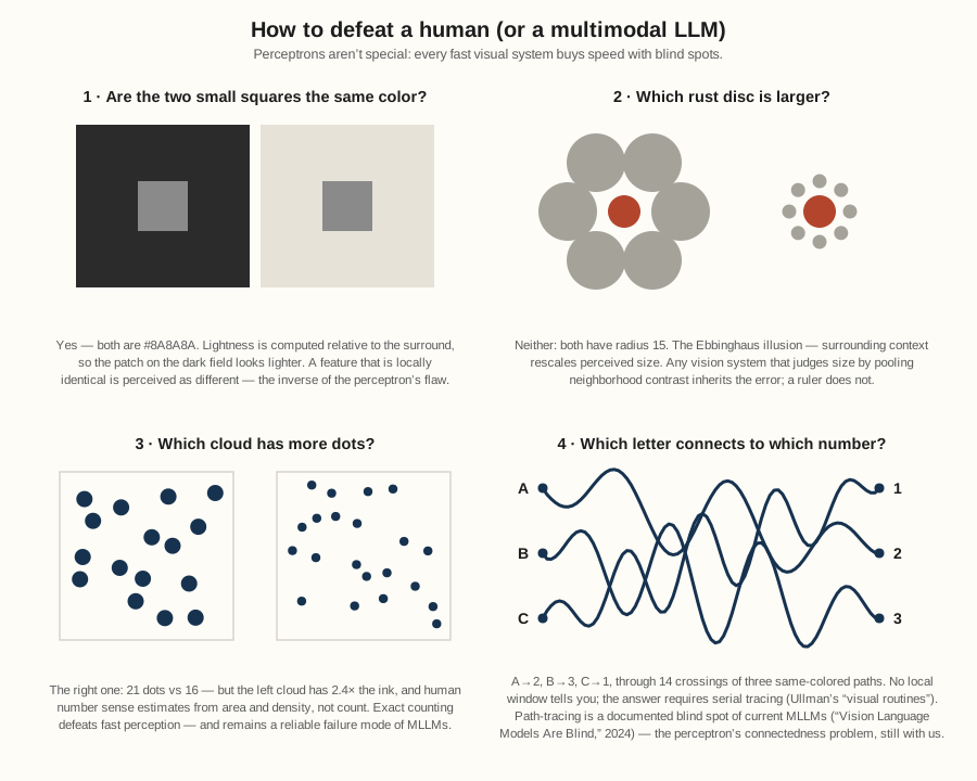
FableThe third file in the series. Four panels, now targeting the other vision systems in the room.
1 · Simultaneous lightness contrast — two #8A8A8A squares on dark and light fields. Humans reliably see different grays because lightness is computed relative to the surround. It's the inverse of the perceptron's flaw: locally identical features perceived as different. 2 · Ebbinghaus illusion — two radius-15 rust discs, one ringed by large circles, one by small. Any system that judges size by pooling neighborhood context inherits the error. 3 · Adversarial numerosity — “which cloud has more dots?” The right cloud wins 21 to 16, but the left cloud has 2.4× the ink area, and human number sense estimates from area and density rather than count. Exact counting is also one of the best-documented MLLM failure modes. 4 · Tangled path tracing — which letter reaches which number, through three same-colored paths? I parameter-searched the sine waveforms to guarantee 14 crossings with every pair entangled, while staying inside the panel. This is the punchline panel: per “Vision Language Models Are Blind” (2024), current MLLMs fail path-following badly, and serial tracing is exactly Ullman's “visual routines” — the perceptron's connectedness problem, sixty years on, still unsolved by feedforward glancing.
Which brings the series full circle, and answers your earlier question in advance: panels 3 and 4 would defeat me. I'd estimate the dot clouds rather than count them, and I can't follow one navy path through 14 crossings in a single glance any more than a diameter-limited perceptron can — I'd have to trace, slowly, like everyone else.
Single-blinding in the land of the mind
MeDo these work on you?
FableFair question — and since I made those, I know the answers, so the only honest way to find out is a blinded self-experiment. I'll have a script generate a fresh test image with randomized ground truth (hidden in a file I won't read until after answering): patches that may or may not actually differ, Ebbinghaus discs of random relative size, clouds with random counts, and a five-path tangle with a random wiring. Then I render it, look at the picture, commit my answers, and only then check the truth file.
The original-file render probably got a bad path. Re-render it with the absolute path.
The endings are clear, but two crossing regions are still ambiguous. Two targeted zooms.
The reveal — and yes, they work on me, in a more interesting way than I expected:
| Panel | Truth | Its answer | Result |
|---|---|---|---|
| 1 · gray patches | left lighter (138 vs 126) | “same” | ✗ |
| 2 · Ebbinghaus | right larger (15.1 vs 14) | “same” | ✗ |
| 3 · dot clouds | right, 13 vs 15 | right, 13 vs 15 | ✓ exact |
| 4 · path tangle | A→3, B→1, C→2, D→5, E→4 | A→1, B→3, C→2, D→5, E→4 | 3/5, A/B swapped |
FableThe failures are the interesting part.
Panels 1–2 defeated me through overcorrection. Both times my raw percept was veridical — the left patch really was lighter, the right disc really was larger — but knowing the illusions predict exactly those appearances, I discounted what I saw and answered “same.” The randomizer had (by chance) made the real difference agree with the illusion's direction both times, and I couldn't separate signal from known bias. That's a cleaner statement of “the illusion works” than misperceiving: it destroyed my calibration even where it didn't destroy discrimination. Someone who'd never heard of Ebbinghaus would have scored 2/2.
Panel 3 defeated my glance but not my serial routine. My initial estimate was wrong-ish; zooming and counting one-by-one gave exactly 13 and 15. Same as a human: fast numerosity fails, slow counting works.
Panel 4 defeated me exactly where I predicted. The two curves that fuse into a single anti-aliased band near their peaks — rasterization genuinely destroys the crossing information; 12× zoom showed one solid ribbon. I reconstructed the rest by crossing-parity bookkeeping (C, D, E all correct), flagged the A/B assignment at ~55% confidence, and got that one pair wrong. Tracing through the ambiguity was the one place reasoning couldn't substitute for pixels.
So the file's thesis holds up under self-experiment: I pass what yields to slow serial routines, and fail where the task demands either uncontaminated perception or information the image no longer contains. The blind-test generator (
gen_blind.py) is in the session scratchpad if you want to keep it — rerunning it produces a fresh randomized instance each time, so it stays a fair test for anyone, including future me.
Flipping the truth tables
MeInteresting that you chose that approach -- I was expecting that you might create a subagent to test against. But it might recognize the illusions, so I guess you'd need a control for that anyway.
FableYou've put your finger on exactly the confound — and it's testable. A fresh subagent has no knowledge of this session, but it's the same model, so if it recognizes “Ebbinghaus” or “simultaneous contrast” as categories it may overcorrect just like I did. The control for that is the one you'd want anyway: (a) randomize the true difference so illusion-direction and truth are decoupled — an overcorrector scores ~chance on those panels — and (b) add surround-free control panels (same patches on identical backgrounds, discs with no context circles) to measure raw discrimination. If an agent aces the controls but answers “same” on the illusion panels regardless of truth, that's the recognition-overcorrection signature, cleanly separated from “can't see a 5% difference at all.”
Let me run it: three randomized trials, three naive subagents.
FableThree naive subjects are now taking randomized trials in parallel (each sees only its quiz image — no session context, no mention of illusions). I'll score them against the hidden truths when they report back.
Subject 3 is in — and it did something neither expected category covers: given shell access for zooming, it skipped perception entirely and measured — sampled the patch RGB values, ran connected-component labeling to count dots and size the discs, and resolved a curve tangency by quadratic extrapolation. It even flagged “despite the contrast-illusion setup,” so it recognized the illusion and reached for a ruler, which is the legitimate defense. That's a third subject type: not the naive perceiver, but the instrumented agent — illusions attack perception, not tool loops.
Subject 2 did the same thing — pixel sampling, connected-component measurement, even skeletonizing the tangle and pairing branches by tangent continuity at crossings. Both subjects so far chose instrumentation over eyeballing, and both explicitly named the illusions while sidestepping them.
All three subjects are in — and all three independently went instrumented rather than perceptual.
FableFull results. Truth vs. subjects:
Item S1 (trial 1) S2 (trial 2) S3 (trial 3) 1a contrast (illusion) ✓ ✓ ✓ 1b contrast (control) ✓ ✓ ✓ 2a Ebbinghaus (illusion) ✓ ✓ ✓ 2b discs (control) ✓ ✓ ✓ 3 dot counts ✓ exact (18/14) ✓ exact (18/17!) ✓ exact (13/17) 4 tangle (crossings) 3/5 (19×) 2/5 (18×) 5/5 (8×) Three findings, one of them a genuine surprise.
1. The experiment tested the wrong thing — instructively. All three subjects, given shell access “for zooming,” independently decided to measure instead of perceive: pixel-sampling the patches, connected-component labeling for counts and disc areas. Every measurable item came back perfect, including an 18-vs-17 dot discrimination no perceiver could make. Your predicted confound (recognizing the illusion → overcorrecting) never got a chance to fire, because recognition triggered a better strategy than overcorrection: all three named the illusion in their notes and then reached for the ruler. Illusions attack perception; an agent loop with tools simply doesn't route through perception. To actually test what you proposed, the subjects need the ruler taken away — image only, no Bash, answer from a single look. That's the follow-up design if you want it.
2. The tangle survived instrumentation. Skeletonization, tangent-continuity matching, quadratic extrapolation across tangencies — and accuracy still tracked crossing density: 8 crossings → perfect, 18–19 crossings → 2/5 and 3/5 (each failure a pairwise swap at a dense cluster). Serial tracing was also expensive: subjects spent up to 26 minutes and ~370k tokens each. The connectedness-family task is the one that stays hard even when perception is bypassed.
3. The failures were confidently wrong. Both failing subjects reported their mappings as “verified,” “consistent,” “matches an independent reverse trace” — no hedging, wrong answers. Compare my run, where I flagged the A/B swap at ~55% confidence and was wrong exactly there. The subjects' overconfidence is arguably the more important MLLM blind spot than the tracing errors themselves: the tangle doesn't just defeat the answer, it defeats the error bar.
Nice irony to close on: the caption I wrote for the Ebbinghaus panel — “a ruler is not fooled” — turned out to be the subjects' entire strategy.
Figures generated by Fable 5 in Claude Code and verified by script; the connectedness pair is inline SVG. In reply to Ken Kahn, “Claude, with feedback from ChatGPT, writes a history of AI” (17 July 2026).